| Citation: | ZHANG Miao, HE Yi-juan, YANG Bo-yu, LUO Zheng-wei, LU Wan-li, TANG Tao, LI Kai-cheng, LYU Ji-dong. Trajectory prediction method for high-speed train group tracking operation based on LSTM-KF model[J]. Journal of Traffic and Transportation Engineering, 2024, 24(3): 296-310. doi: 10.19818/j.cnki.1671-1637.2024.03.021

|
As the brain and central nervous system of the high-speed railway system, the train operation control system (referred to as the train control system) plays a crucial role in ensuring the safe and efficient operation of trains[1]At present, typical train control systems used in high-speed railways include the Chinese Train Control System (CTCS) Level 3 and CTCS Level 2, the European Train Control System (ETCS), and Japan's Automatic Train Control (ATC), all of which operate in a fixed block control mode[2]To meet the growing demand for passenger transportation, the operating density of high-speed railway trains is constantly increasing, and the existing operating intervals are approaching the design limit of the system. Based on fixed block system[3]The train control technology is difficult to meet the demand for further improving operational efficiency of high-speed railways. At present, achieving high-speed train group operation in existing networks is an important technical means to further shorten train operation intervals and improve system capacity, and is the core and key to the development of railways at home and abroad[4].
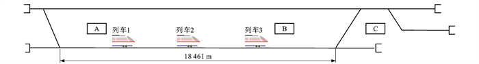
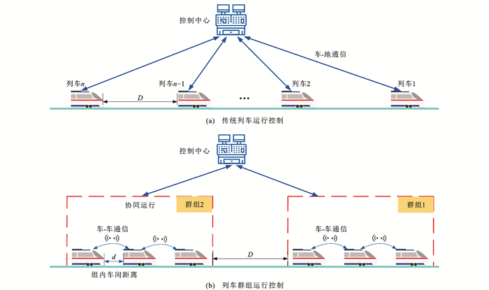
In the operation control of high-speed train groups,nHeterogeneous trains will be interconnected through train to train communication, and operate in a coordinated and safe manner with shorter tracking distances under the constraints of the track. This is an important feature that distinguishes train group operation from traditional train operation[5]Vehicle to vehicle communication technology plays a crucial role in building group operations. The basic principles of group operation control and its differences from traditional train operation control are as follows:Figure 1As shown, the tracking interval of trains under traditional train operation control and the inter group interval of group operation are bothDTrain tracking interval within the groupdClearly less thanDCompared with the traditional train operation control mode, multiple heterogeneous trains in a train group share real-time speed, position, acceleration, internal status and other information of train operation through train to train communication technology, thereby coupling to form an organic whole, which further reduces the tracking interval of the train group while ensuring safe and smooth operation[6]However, the smooth operation of high-speed train groups is affected by the limited short distance signal transmission capacity and time-varying signal quality of train to train communication technology[7]How to maximize the role of vehicle to vehicle communication technology and enhance the smoothness of formation operation is still an urgent problem to be solved. In order to reduce the impact of vehicle to vehicle communication delay, predicting the trajectory of the preceding vehicle within the group is an important means to further reduce the tracking distance of trains.

There is relatively little research on train trajectory prediction theory both domestically and internationally. He and others[8]A subway train trajectory prediction method based on Long Short Term Memory (LSTM) network was proposed, and simulation experiments were conducted using actual train operation data. The results showed that the LSTM model had better long-term prediction accuracy than the Kalman Filter (KF) model; Yin et al[9]The LSTM model combined with time delay information was used to predict the running trajectory of high-speed trains, and the effectiveness of the method was verified through simulation. Obviously, current research on train trajectories focuses on data-driven prediction methods.
It is worth noting that many scholars have conducted in-depth research on vehicle trajectory prediction and urban traffic flow prediction. The trajectory prediction methods used mainly include short-term physical model-based trajectory prediction and data-driven trajectory prediction. The trajectory prediction method based on physical models is to predict the changes in the vehicle's state over a period of time based on the relevant kinematic and dynamic laws of the vehicle. Lin et al[10]Based on a two degree of freedom dynamic model, the future trajectory of the vehicle is predicted. In order to improve the accuracy of trajectory prediction, the author proposes a stable KF method to estimate the lateral velocity of the vehicle and external disturbances acting on the vehicle; De Miguel and others[11]Using the recursive layer and variational autoencoder architecture model of deep learning for future local trajectories, it has been experimentally proven to achieve good results; Wang et al[12]After comparing a large number of statistical models and deep learning models, it was concluded that the hybrid model of LSTM combined with random forest has better predictive performance; Lytrivis et al[13]Considering the position, velocity, and heading angle of all surrounding vehicles, a kinematic model based on constant yaw rate and constant acceleration is used to collaboratively calculate the future position changes of the vehicles. At the same time, based on map information, the trajectory prediction effect is enhanced; Zhou Bing and others[14]Predicting train trajectories based on motion models and considering the uncertainty of motion trajectories to make decisions on braking and collision avoidance for high-speed vehicles. This method can judge the probability of future collisions, but in high-speed situations, a single motion model prediction method can cause significant errors in the later stages of motion; Tong et al[15]The Transformer model was used to predict and evaluate long-term trajectories, achieving good results; Reiter et al[16]A quadratic programming algorithm was proposed for the most challenging motion planning problems in both long and short-term time ranges, and achieved good results in motion planning problems; Huang et al[17]Based on differential positioning navigation system, different kinematic trajectory prediction models were studied, and it was pointed out that the main sources of error in kinematic trajectory prediction are changes in driving intention and behavior; Zhang Miao and others[18]Propose intelligent train control methods based on driver experience; Sorstedt et al[19]By considering the driver's control input, predict the driving trajectory for a period of time in the future. It can be seen that traditional trajectory prediction often uses a single motion model, and different motion models achieve different trajectory prediction results. However, the actual driving process of vehicles is very complex, which makes it difficult for any single motion model to accurately describe the motion state of the vehicle at any time. For feature extraction problems in complex environments, Xu et al[20]A cascaded feature LSTM model was proposed, which can extract complex interaction feature information between pedestrians; Li et al[21]A clustering convolutional LSTM algorithm was proposed for predicting vehicle trajectories, and experiments showed that the extraction of interactive information and selected features was accurate and met real-time requirements.
The vehicle trajectory prediction method based on data-driven methods mainly uses a large number of data sequences and data-driven models (such as deep learning network models) to predict the future driving trajectory of vehicles by learning and mining knowledge from the data. The data-driven vehicle trajectory prediction method is mainly based on the trajectory prediction model of deep learning network, which predicts the driving trajectory by considering the relationship and influence of time and spatial variables. Xing et al[22]The Gaussian mixture model was used to recognize driving styles, and LSTM network and Recurrent Neural Network (RNN) were used to predict the trajectory of vehicles ahead, achieving good results; Kim and others[23]Based on the long short-term memory model in recurrent neural networks, analyze the temporal behavior of vehicles in traffic environments and predict their future driving trajectories. Compare and analyze the predicted results with commonly used KF based methods. The trajectory prediction method based on deep neural network learning models can predict vehicle trajectories for a longer period of time, but it requires a higher database; Dequaire et al[24]A recurrent neural network was used to describe the temporal and spatial changes in the traffic environment, and a unified motion tracking and prediction learning model for traffic participants such as vehicles and pedestrians was constructed; Xie et al[25]After comparing multiple prediction models, a sequence prediction model combining LSTM and particle swarm optimization algorithm was proposed, and its accuracy was demonstrated through experiments; Deo et al[26]The LSTM method was used to predict the trajectory of vehicles around highways; Zhao et al[27]A traffic flow prediction model based on LSTM was proposed, with the motivation of utilizing a two-dimensional network composed of memory units in LSTM to simultaneously consider the spatiotemporal correlation of traffic sequence information, and the model was verified to have better predictive performance.
Unlike existing research, this paper proposes a novel hybrid model that integrates data-driven LSTM models and physics based KF models to predict train trajectories. In the proposed LSTM-KF hybrid model, the LSTM model is used to analyze time series data and explore the long-term dependencies of train trajectory data, which can be assumed to be the observation data of the KF model. The KF model combines the train dynamics mechanism to extract local features of train operation data, thereby smoothing the train trajectory predicted by the LSTM model. In addition, this article designs a real-time algorithm that can effectively implement the LSTM-KF hybrid model, relying on the high-speed railway control system simulation testing platform of Beijing Jiaotong University, and conducting simulation experiments using standard line data designed based on actual railway conditions in China.
In order to more accurately describe the problems in the process of high-speed train trajectory prediction, the following definitions are made.
Definition (Train Trajectory)[8]During the one-way operation of high-speed trains, the changes in train position and speed along the track can be considered as longitudinal variables. The train trajectory within a certain period of time can be represented as
|
XN,t={st,vt,⋯,st+N−1,vt+N−1} |
(1) |
In the formula:XN, tStarting from timet, including continuousNTrain trajectory at a sampling time;stFor the momenttCorresponding train position;vtFor the momenttCorresponding train speed.
Generally, historical train operation data can be represented as
|
ON,h,t={st−N+1,vt−N+1,ut−N+1,⋯,st,vt,ut} |
(2) |
|
SN, h,t={st−N+1,⋯,st} |
(3) |
|
VN, h,t={vt−N+1,⋯,vt} |
(4) |
In the formula:ON, h, tTo terminate attTime, including continuityNTrain historical operation data at each sampling moment;utFor the momenttCorresponding train control commands;SN, h, tTo terminate at timet, including continuousNThe position sequence in the historical train operation data at each sampling time;VN, h, tTo terminate attTime, including continuityNThe speed sequence in the historical train operation data at each sampling time.
The train trajectory prediction model can be represented as a mapping function for historical operating data[9]That is
|
ˆXM,p,t=Φ(ON, h,t) |
(5) |
|
ˆXM,p,t={ˆst+1,ˆvt+1,ˆst+2,ˆvt+2,⋯,ˆst+M,ˆvt+M} |
(6) |
In the formula:ˆXM,p,tStarting from timet+1, including continuousMThe final predicted train trajectory output at each sampling moment, whereMAlso known as historical time steps;Φ(⋅)Mapping function from historical train trajectories to predicted train trajectories;ˆst+1Based on the current situationtTime predictiont+1Train position at time;ˆvt+1Based on the current situationtTime predictiont+1Train speed at the moment.
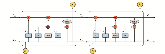
LSTM network is a variant of RNN network with a gate mechanism for capturing long-term dependencies[28]LikeFigure 2As shown, The basic component of an LSTM network is a memory block consisting of a forget gate, an input gate, and an output gate. During the continuous data reception process, the memory block maintains a unit state to store historical informationCtexpress. The two inputs of the memory block are the current statextOutput from the previous sequenceht−1The memory block will replace the previous oneht−1Compared to the current statextCombined together, astActual input vector at the moment(ht−1,xt)Then, the combined input vector is used to calculate the output through three gateshtAnd update the cell state toCt.

The basic formula is
|
{ft=σ[Wf(ht−1,xt)+bf]it=σ[Wi⋅(ht−1,xt)+bi]Ct=ft∗Ct−1+it∗tanh[WC(ht−1,xt)+bC]ot=σ[W∘⋅(ht−1,xt)+bo]ht=ot∗tanh(Ct) |
(7) |
In the formula:ftTo forget the doortOutput of time;σTo activate the function;itFor the input gate intOutput of time;οtFor the output gatetTime output;Wf、Wi、WC、WoThe weight matrix in the memory block corresponding to each gate;bf、bi、bC、boThe deviation matrices in the memory blocks corresponding to each gate* For convolution operation.
KF is a prediction model based on linear regression, which uses the state space of linear stochastic systems to describe it[29]The KF model can be divided into two parts: prediction and update, where the prediction equation is
|
ˆxt+1∣t=Ft+1ˆxt∣t+Bt+1ut |
(8) |
|
Pt+1∣t=Ft+1Pt∣tFTt+1+Qt+1 |
(9) |
In the formula:ˆxt+1∣tBased on the current situationtTime predictiont+1The state of time;Bt+1To control the matrix and reflectt+1Time system control inpututThe impact;Ft+1dot+1Time state transition matrix;Pt+1∣tBased on the current situationtObtained at all timest+1Time prediction error covariance matrix;Qt+1dot+1Covariance matrix of time system noise.
The update equation in the KF model can be expressed as
|
Kt+1=Pt+1∣tHTt+1(Ht+1Pt+1∣tHTt+1+Rt+1)−1 |
(10) |
|
ˆxt+1∣t+1=ˆxt+1∣t+Kt+1(zt+1−Ht+1ˆxt+1∣t) |
(11) |
|
Pt+1=(I−Kt+1Ht+1)Pt+1∣t |
(12) |
In the formula:Kt+1dot+1Kalman gain at time;Ht+1dot+1The time mapping matrix maps the state vector to the observed values;Rt+1dot+1Observing noise at all times is the variance of the standard normal distribution;zt+1dot+1Observation values of time;Pt+1dot+1Covariance matrix of prediction error at time.
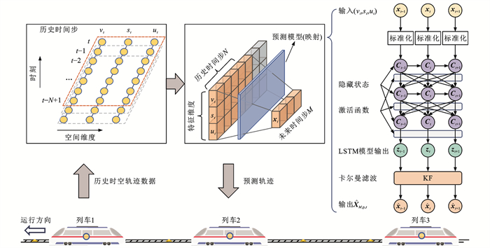
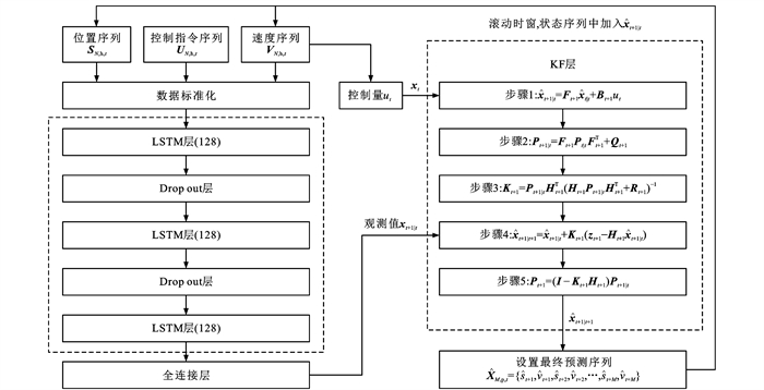
in compliance withFigure 3As shown, taking Train 1 (front car) and Train 2 (rear car) as examples, the principle of train trajectory prediction based on LSTM-KF hybrid model is explained as follows: current timetTrain 2 combines the historical spatiotemporal trajectory data of Train 1 (historical time steps)N)Using the LSTM model to predict the next state of Train 1 in the long time domain (i.e. the assumed observation data of the KF model)zt+1), and capture corresponding reference control action informationutThen filter the state information predicted by the LSTM model through the KF model to generate more accurate estimatesˆxt+1∣t+1Next, we willˆxt+1∣t+1At the end of the input sequence of the LSTM model, update the input sequence and repeat the aforementioned rolling prediction steps until the final length of the prediction time step is obtainedMThe predicted trajectory; At this point, Train 2 has completed the current tasktPredict the trajectory of train 1 ahead at the given time.

Define the train operation status as
|
xt=[stvt] |
(13) |
A specific LSTM model has been designed for predicting train trajectoriesL(·), its structure is as followsFigure 4As shown, the corresponding function can be expressed as the following function
|
X1,p,t=L(XN, h,t,UN, h,t) |
(14) |
|
X1,p,t=(xt+1∣t) |
(15) |
|
XN, h,t=(xt−N+1,xt−N+2,⋯,xt) |
(16) |
|
UN, h,t=(ut−N+1,ut−N+2,⋯,ut) |
(17) |
In the formula:X1,p,tBased on the modelL(∙)Predictedt+1The current train status corresponds to the predicted time step1;XN, h,tTo terminate at timet, including continuousNHistorical state data at each sampling moment;UN, h,tTo terminate at timet, including continuousNHistorical acceleration data at each sampling moment.
It is worth noting that the "historical" data may not necessarily be the actual operation data of the train, and may also be the predicted values output by the LSTM-KF hybrid model. For example, the current time ist, The LSTM-KF hybrid model has already rolled out the prediction outputt+The train status value at time 1 is relative tot+In terms of the state predicted by the model after 1 moment, it is' historical 'data.
Furthermore, future control behavior data of the preceding vehicle is extracted through differential calculation, i.e
|
UM,p,t=(ut∣t,ut+1∣t,⋯,ut+M−1∣t) |
(18) |
|
ut+i∣t={uti=0vt+i+1∣t−vt+i∣tΔτ1⩽i⩽M−1 |
(19) |
In the formula:UM,p,tStarting from timet, including continuousMThe future reference control sequence of the preceding vehicle at each sampling moment;ut+i∣tBased ontTime predictiont+iFuture reference control behavior of the vehicle before the time;vt+i∣tPredicting trajectories for LSTM modelsUM,p,tpass the civil examinationsiTrain speed at one time step;ΔτFor the sampling interval.
For high-speed trains, the approximate expression of the dynamic equation is[29]
|
{ˆst+1∣t=ˆst∣t+ˆvt∣tΔτ+utΔτ22ˆvt+1∣t=ˆvt+1∣t+Δτut |
(20) |
Equation (20) is used as the prediction equation of the KF model for train trajectory prediction, whereˆxt+1∣tandˆxt∣tCan be defined as(ˆst+1∣t,ˆvt+1∣t)Tand(ˆst∣t,ˆvt∣t)T(or(ˆst,ˆvt)T)Afterwards, a complete KF model can be constructed according to the steps in section 2.2. The structure of the KF model is as followsFigure 4As shown, the corresponding parameters are as follows
|
Ft+1=[1Δτ01] |
(21) |
|
Bt+1=[Δτ22Δτ] |
(22) |
|
Ht+1=[1001] |
(23) |
Based on the above ideas, this article proposes a train trajectory prediction algorithm based on the LSTM-KF hybrid model, which can predict the current train trajectory at a given timetAccurately predict and output the futureMThe train trajectory at a certain moment. The train trajectory prediction algorithm has two advantages: (1) the algorithm uses the LSTM model to learn the rules of the train's historical trajectory, and uses the train operation mechanism included in the KF model to correct the trajectory prediction value, which enhances the interpretability of the model while achieving high-precision train trajectory prediction; (2) Complex LSTM models can be trained offline, while KF models themselves are lightweight, and the combination of the two can make the algorithm easy to deploy in real-time online.
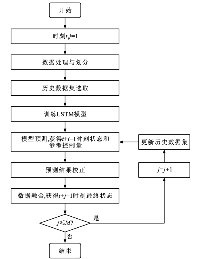
The process of train trajectory prediction algorithm based on LSTM-KF model is as follows:Figure 5As shown.

Firstly, fromtStart predicting the timing and initialize the stepsjTo 1, organize the collected data of train operation, select data from longer operating stages, and calculate estimated data to supplement the discontinuous collected data during the selected stages. Set the training dataset and validation dataset in a certain proportion, and normalize the data to prevent large-scale data from having a significant impact on small-scale data. Secondly, select the latest set of data from the training dataset as historical data. Next, build an LSTM model and train it using training data to extract the motion patterns during train operation. Fix the model parameters after convergence.
Use LSTM model to predict historical data sets. In the prediction result correction section, the KF model is used to correct the prediction results of the test model. Normalize the output of LSTM, linearly calculate the train state data according to the train dynamics equation, and use the covariance matrix to correct the linearly calculated train state. Then, linearly combine the predicted data of the LSTM model with the KF calculation results. Finally, normalize the fused data, include it in the latest data position of the historical dataset, and remove the oldest data to complete the rolling update.
This article relies on the laboratory high-speed railway control system simulation testing platform, and the line is tested using standard line data designed based on the actual line conditions of Chinese railways, such asFigure 6As shown, it consists of three standard station areas: A, B, and C. The case study of trajectory prediction is carried out by taking the three detection characteristics (position, speed and control command) directly collected by the train auto drive system in the simulation test platform as the input of the prediction model.
The data is recorded by the Juridical Recording Unit (JRU) in the vehicle, with a sampling interval of ΔτFor 0.5 seconds, perform the following 5 preprocessing operations on the data.
(1) Missing data points are filled with a combination of historical mean and pre - and post values.
(2) The distance traveled by the train within the unit sampling interval is calculated by subtracting the train positions at the previous and next time points.
(3) After checking for missing and invalid data, standardize each dimension feature.
(4) Acceleration is estimated using velocity and sampling interval.
(5) Historical data is processed into a data with historical time stepsNA prediction dataset with a scrolling window step size of 1. For the convenience of comparing and verifying the training effect of the model, 80% of the data is selected for training, and the remaining 20% is used for testing.
This article usesZ-Score normalization is used to scale features with typical normal distribution attributes, with a mean of 0 and variance of 1, to standardize the data.
The specific configuration of constructing a LSTM-KF hybrid model for train trajectory prediction includes loss function, activation function, optimization algorithm, and parameter settings to ensure the accuracy and convergence of the model.
(1) Loss function
Measure the degree of deviation between the predicted and actual values of the model using a loss function. The better the loss function, the better the performance of the model. In order to measure the Euclidean distance error of each trajectory while considering regression problems, this paper uses Mean Square Error (MSE), i.e
|
E=1nn∑i=1(yi−ˆyi)2 |
(24) |
In the formula:EMean square error;yiFor the thkStep true value;ˆyiFor the thkStep prediction value;nFor the total time step.
(2) Activation function
This article uses the Rectified Linear Unit (ReLU) function as the activation function for train operation status. This function solves the gradient vanishing problem, and compared to Sigmoid and tanh, ReLU has faster computation and convergence speed.
(3) Optimization algorithm
The convergence of deep learning models is highly dependent on the selected optimizer. The Adaptive Moment Estimation (ADAM) algorithm is suitable for problems with large amounts of data or parameters because it has high computational efficiency, requires minimal memory, and is invariant to rescaling the diagonals of gradients. Therefore, this paper uses an ADAM optimizer to construct the model on each train trajectory dataset.
(4) Parameter settings
The parameters of the prediction model are as followsTable 1As shown, the historical time step N refers to a single sample in the historical data that contains the pastNThe state and control variables at each moment, predicting the time step sizeMIt refers to predicting trajectories that include the futureMThe state of a moment. In particular, LSTM networks with different structures are tested, such as the number of LSTM layers and the number of hidden units in each layer, and KF observation covariance matrix is adjusted in the experimentQCovariance matrix of process errorR.
| 参数 | 取值 |
| LSTM网络结构 | 100×100 |
| 预测时窗/s | 6 |
| 历史时间步长 | 12 |
| 未来时间步长 | 30 |
| 状态迁移矩阵 | [00.501] |
| 观测矩阵 | [1001] |
| 观测协方差矩阵 | [100010] |
| 过程误差协方差矩阵 | [0.1000.1] |
 DownLoad:
CSV
DownLoad:
CSV
Compare the trajectory prediction results of various models using three metrics: Root Mean Square Error (RMSE), Mean Absolute Error (MAE), and Mean Absolute Percentage Error (MAPE)E1、E2、E3show
|
E1=√1nn∑i=1(yi−ˆyi)2 |
(25) |
|
E2=1nn∑i=1|yi−ˆyi| |
(26) |
|
E3=1nn∑i=1|yi−ˆyiyi| |
(27) |
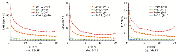
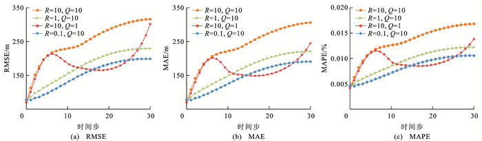
After fixing the parameters of the LSTM model, exploreR、QThe impact of two covariance matrices on the prediction results is adjusted by adjusting the covariance of the KF model observation matrixRCovariance of Process Error MatrixQrealization. According to equation (10), the Kalman gain andR、QThe ratio of matrix coefficients is related. For the convenience of evaluationR、QThe function of a matrix is toR、QEqual to multiplying the identity matrix by constant coefficientsR、QAfterwards, design experimentsR/Qrespectively0.01、0.1、1、10Four different situations to exploreR、QThe impact of both on the prediction results.
Figure 7The results of the LSTM-KF model for predicting train speed indicate that:R=Q=At 10 o'clock, the RMSE and MAE evaluation index values gradually decreased from around 48 on the vertical axis, indicating a large initial prediction error. As the rolling prediction progressed, the predicted values gradually approached the actual values; existR=1 andQ=At 10 o'clock, the speed prediction value of the LSTM-KF model is more biased towards the prediction value of the LSTM model. In addition, the three indicators RMSE, MAE, and MAPE decrease with increasing time steps, especially after the 18th time step when they tend to stabilizeR/QThe LSTM-KF model performs well in prediction; equalR=10 andQ=At 1 o'clock, the predicted values of the LSTM-KF model tend to be more biased towards the predicted values of the KF model prediction equation, resulting in poorer prediction performance; equalR=0.1 andQ=At 10 o'clock, compared to othersR/QThe RMSE, MAE, and MAPE indicators corresponding to the LSTM-KF model are relatively small and stable.

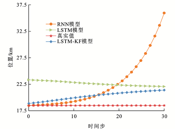
Figure 8The results of the LSTM-KF model for predicting train position indicate that:R=10 andQ=The curves of the three evaluation indicators at 1 hour slowly increase over time and tend to stabilize; From the speed and position prediction results,R=10 andQ=The parameter setting of 1 can enable the LSTM-KF model to achieve better prediction performance. Therefore, chooseR=0.1 andQ=The covariance matrix of 10 is used as a parameter for the LSTM-KF model in subsequent experiments.

In order to verify the performance of the proposed model, data was collected on the high-speed rail control system simulation testing platform of Beijing Jiaotong University. The data was divided into a training set and a testing set, and the model was trained on the training set and validated on the testing set.
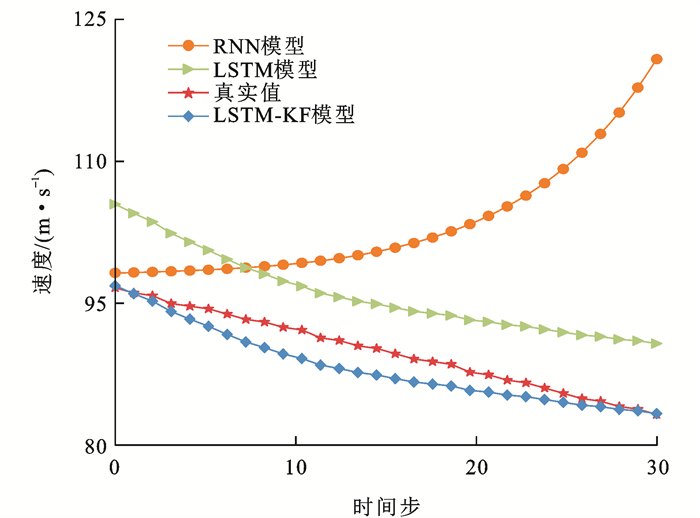
Figure 930 time step train speed curves and actual train speed values predicted by different models under cruising conditions. This experiment compared the performance of LSTM, RNN, and LSTM-KF in 30 step prediction. During the experiment, the last 12 sets of training data (historical data) were taken to predict the first set of data (future data), and then the last 11 sets of training data (historical data) and the predicted data (the first set of future data) were merged into 12 data sets to predict the second set of data in the future. Further realizing the rolling prediction process.
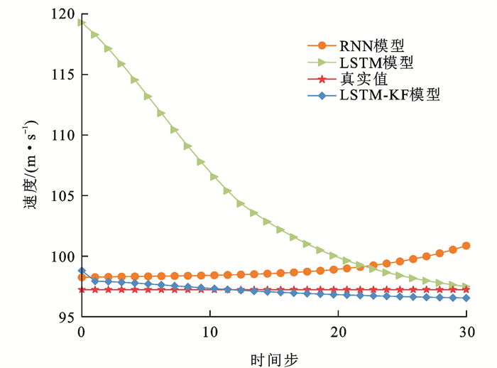
causeFigure 9It can be seen that a single LSTM model has low accuracy in speed prediction, manifested as a true speed of 97 m · s-1The predicted value is 119 m · s-1, with a difference of 22 m · s-1The RNN model is relatively accurate, with predicted values near the true value, which is 97 m · s-1The predicted value is 98 m · s-1, with a difference of 1 m · s-1The LSTM-KF model predicts that the distance between the velocity trajectory and the true value is relatively small, with a true value of 97 m · s-1The predicted value is 98 m · s-1, with a difference of 1 m · s-1The predicted trajectory shows that the model has good predictive performance.
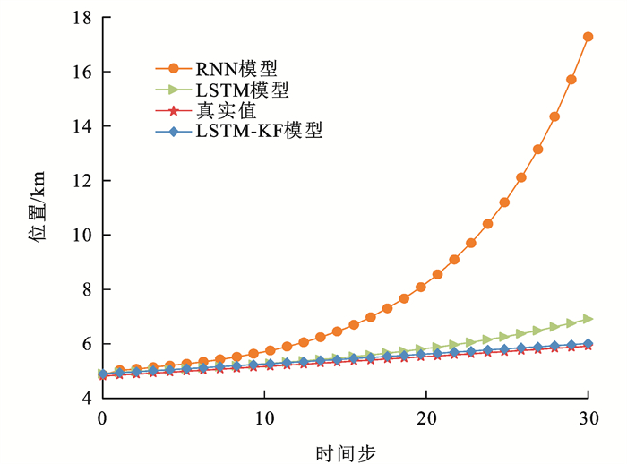
Figure 10For the prediction of train position and the actual value of train position by different models, it can be seen that a single LSTM model has a large prediction deviation for position, with a predicted value of 12171 m and an actual value of 11373 m, a difference of 798 m; The RNN model's prediction of location is not ideal, with a predicted value of 10462m and a true value of 11373m, a difference of 911m; The LSTM-KF model is relatively accurate in predicting location, with a predicted value of 17121 m and a true value of 17043 m, a difference of 78 m.
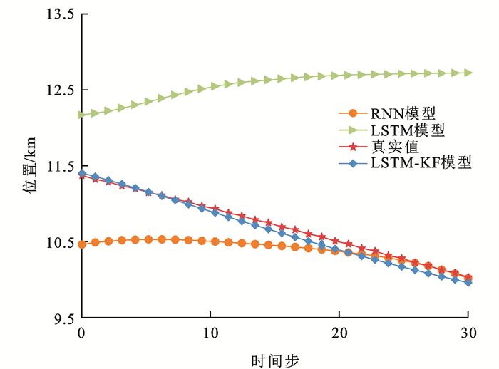
Figure 11The reason why the predicted results of the LSTM-KF model are different from those of the LSTM model with the same parameters for the acceleration predicted by different models and the actual value of train acceleration is that the acceleration is calculated by dividing the difference between the speed values predicted by the two LSTM models before and after by the time interval between the two predictions. Similarly, due to the addition of a fully connected network model, there are certain connections between various features. Therefore, it is normal for the corrected data values of the KF model to have an impact on the prediction results of some other features. causeFigure 11It can be seen that the LSTM model is more accurate in predicting acceleration; The RNN model and LSTM-KF model are inaccurate in fitting acceleration.
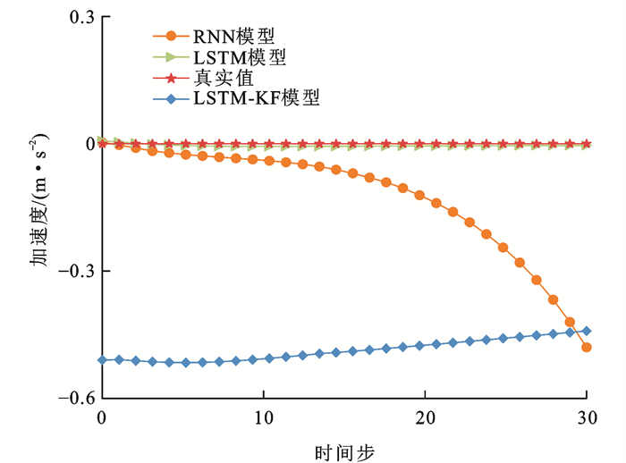
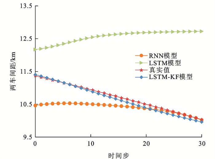
Figure 12It can be concluded that the LSTM-KF model performs well in predicting the distance between two vehicles and their true values for different models, and is close to the true values; The RNN model has a good fitting effect on the indicator of distance from the preceding vehicle, with a large starting point error, and the error gradually decreases with time; The LSTM model does not have ideal fitting effect on the indicator of distance from the preceding vehicle, and the prediction deviation is relatively large.

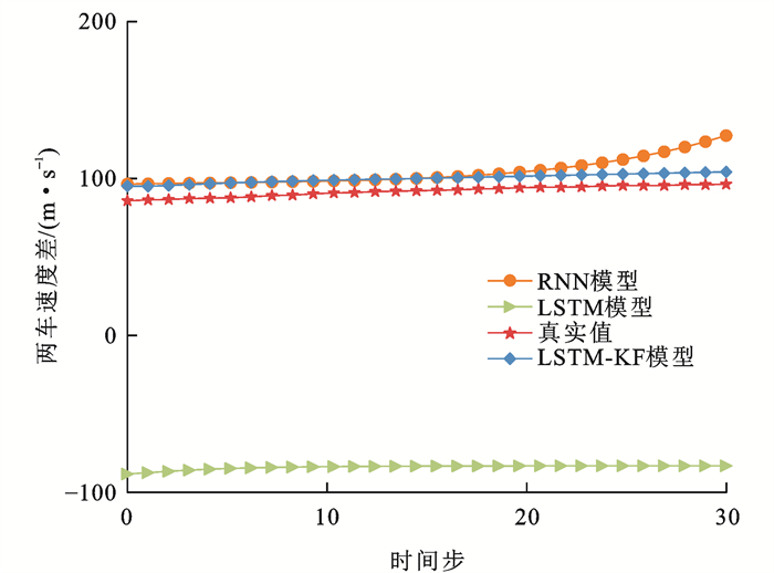
Figure 13It can be seen that the RNN model and LSTM-KF model are more accurate in predicting the speed difference between two vehicles and their true values for different models, but the prediction results of a single LSTM model are not very ideal. For the problem of initial value deviation in other models without KF filtering algorithm for correction, after analysis, it is believed that the reason is that predicting multiple dimensions of data at the same time causes interference in the calculation process of the loss function of key data in different dimensions (such as non critical data such as the speed of the preceding vehicle), such as position prediction. The range of position is 0-12 km, which is normalized to 0-1 by conventional methods, while the range of speed difference is -100~100 m · s-1For the loss function, a speed change of 1 m · s-1The weight is 1/200, and the same weight is required for a position of 60 meters. Therefore, in multidimensional prediction models, a combination of data models and mechanistic models can be used to correct the predicted values of key data (such as velocity and position) through mechanistic models, reducing the errors of key data within an acceptable range.

Table 2For several common evaluation metrics for position prediction using different models, it can be seen that, taking RMSE as an example, in the comparison of multidimensional output prediction models, the RMSE metric of the LSTM-KF model is 7% of that of the traditional LSTM model and 15% of that of the traditional RNN model.
| 时间步 | RMSE/m | MAE/m | MAPE/% | ||||||
| RNN | LSTM-KF | LSTM | RNN | LSTM-KF | LSTM | RNN | LSTM-KF | LSTM | |
| 1 | 1 456.41 | 78.95 | 2 799.74 | 1 456.41 | 78.95 | 2 799.74 | 0.08 | 0.00 | 0.14 |
| 5 | 1 591.03 | 97.88 | 2 464.24 | 1 586.20 | 96.49 | 2 453.65 | 0.08 | 0.01 | 0.12 |
| 10 | 1 904.61 | 132.90 | 2 234.40 | 1 870.70 | 127.31 | 2 211.47 | 0.10 | 0.01 | 0.11 |
| 15 | 2 431.12 | 163.92 | 2 083.96 | 2 311.75 | 155.26 | 2 053.49 | 0.12 | 0.01 | 0.11 |
| 20 | 3 345.82 | 185.87 | 1 961.03 | 3 011.15 | 176.17 | 1 921.79 | 0.14 | 0.01 | 0.10 |
| 25 | 4 966.02 | 196.82 | 1 850.34 | 4 144.52 | 187.91 | 1 799.06 | 0.18 | 0.01 | 0.09 |
DownLoad:
CSV
Table 3For several common evaluation metrics for speed prediction in multiple models, it can be seen that taking RMSE as an example, the speed prediction results under cruising conditions show that the RMSE evaluation metric of the LSTM-KF model is 14% of that of the traditional LSTM model and 30% of that of the traditional RNN model.
| 时间步 | RMSE/(m·s-1) | MAE/(m·s-1) | MAPE/% | ||||||
| RNN | LSTM-KF | LSTM | RNN | LSTM-KF | LSTM | RNN | LSTM-KF | LSTM | |
| 1 | 1.02 | 1.58 | 22.07 | 1.02 | 1.58 | 22.07 | 0.01 | 0.02 | 0.19 |
| 5 | 1.16 | 0.85 | 19.28 | 1.15 | 0.77 | 19.17 | 0.01 | 0.01 | 0.16 |
| 10 | 1.40 | 0.65 | 16.40 | 1.37 | 0.53 | 15.87 | 0.01 | 0.01 | 0.14 |
| 15 | 1.76 | 0.55 | 14.08 | 1.68 | 0.40 | 12.93 | 0.02 | 0.00 | 0.12 |
| 20 | 2.34 | 0.51 | 12.40 | 2.13 | 0.39 | 10.64 | 0.02 | 0.00 | 0.10 |
| 25 | 3.31 | 0.51 | 11.16 | 2.83 | 0.42 | 8.87 | 0.03 | 0.00 | 0.08 |
DownLoad:
CSV

Figure 15To accelerate the prediction results and their true values of different model speeds under different operating conditions, it can be seen that the LSTM model has a large deviation, while the RNN model's prediction results are more accurate. This is related to the different data weights used in multidimensional data prediction. A decrease in the error of one dimension may lead to an increase in the error of other dimensions, while the LSTM-KF hybrid model has better prediction performance.
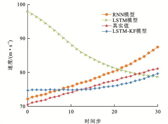

Figure 17To compare the speed prediction results of different models under deceleration conditions with the actual values, it can be concluded that the LSTM model and LSTM-KF model have more accurate prediction results for the data, and the predicted values of the starting and ending points of the LSTM-KF model are relatively close. Therefore, overall, the KF model has a good corrective effect on the prediction results of the LSTM model, while the RNN model is more prone to gradient explosion and requires the addition of more optimization methods such as gradient pruning.

Table 4Based on the actual values of acceleration and deceleration conditions and the predicted values of the LSTM-KF model, the following conclusions can be drawn.
| 时间步 | 加速工况-位置/m | 加速工况-速度/(m·s-1) | 减速工况-位置/m | 减速工况-速度/(m·s-1) | ||||
| 真实值 | LSTM-KF模型预测值 | 真实值 | LSTM-KF模型预测值 | 真实值 | LSTM-KF模型预测值 | 真实值 | LSTM-KF模型预测值 |
|
| 1 | 4 806.00 | 4 892.41 | 70.56 | 74.69 | 18 499.00 | 18 894.95 | 96.67 | 96.88 |
| 2 | 4 806.00 | 4 892.41 | 71.11 | 74.89 | 18 519.00 | 18 983.17 | 96.11 | 96.03 |
| 3 | 4 849.00 | 4 936.37 | 71.39 | 74.89 | 18 499.00 | 19 082.20 | 95.83 | 95.25 |
| 4 | 4 877.00 | 4 964.85 | 71.67 | 74.87 | 18 519.00 | 19 189.04 | 95.00 | 94.16 |
| 5 | 4 949.00 | 5 037.90 | 71.94 | 74.82 | 18 499.00 | 19 300.63 | 94.72 | 93.36 |
| 6 | 4 992.00 | 5 081.46 | 72.50 | 74.97 | 18 517.00 | 19 414.51 | 94.44 | 92.60 |
| 7 | 5 021.00 | 5 111.03 | 72.78 | 74.90 | 18 499.00 | 19 529.68 | 93.89 | 91.75 |
| 8 | 5 065.00 | 5 155.61 | 73.06 | 74.84 | 18 517.00 | 19 644.79 | 93.33 | 90.96 |
| 9 | 5 094.00 | 5 185.20 | 73.61 | 74.95 | 18 498.00 | 19 759.37 | 93.06 | 90.37 |
| 10 | 5 138.00 | 5 229.78 | 73.89 | 74.89 | 18 517.00 | 19 872.41 | 92.50 | 89.69 |
| 11 | 5 168.00 | 5 260.35 | 74.17 | 74.83 | 18 497.00 | 19 983.59 | 92.22 | 89.22 |
| 12 | 5 212.00 | 5 304.92 | 74.72 | 74.98 | 18 517.00 | 20 092.02 | 91.39 | 88.53 |
| 13 | 5 242.00 | 5 335.48 | 75.00 | 74.95 | 18 497.00 | 20 197.32 | 91.11 | 88.16 |
| 14 | 5 287.00 | 5 381.00 | 75.28 | 74.99 | 18 515.00 | 20 294.13 | 90.56 | 87.74 |
| 15 | 5 317.00 | 5 411.49 | 75.56 | 75.04 | 18 498.00 | 20 388.78 | 90.28 | 87.49 |
| 16 | 5 363.00 | 5 457.98 | 76.11 | 75.30 | 18 515.00 | 20 480.60 | 89.72 | 87.10 |
| 17 | 5 393.00 | 5 488.45 | 76.39 | 75.39 | 18 496.00 | 20 569.20 | 89.17 | 86.74 |
| 18 | 5 439.00 | 5 534.91 | 76.94 | 75.69 | 18 515.00 | 20 654.33 | 88.89 | 86.53 |
| 19 | 5 470.00 | 5 566.35 | 77.22 | 75.82 | 18 496.00 | 20 735.88 | 88.61 | 86.33 |
| 20 | 5 516.00 | 5 612.77 | 77.50 | 75.98 | 18 514.00 | 20 813.79 | 87.78 | 85.86 |
| 21 | 5 547.00 | 5 644.17 | 77.78 | 76.15 | 18 496.00 | 20 888.06 | 87.50 | 85.68 |
| 22 | 5 594.00 | 5 691.55 | 78.33 | 76.54 | 18 513.00 | 20 958.73 | 86.94 | 85.37 |
| 23 | 5 625.00 | 5 722.92 | 78.61 | 76.77 | 18 496.00 | 21 025.86 | 86.67 | 85.20 |
| 24 | 5 672.00 | 5 770.26 | 78.89 | 77.03 | 18 512.00 | 21 089.52 | 86.11 | 84.90 |
| 25 | 5 704.00 | 5 802.59 | 79.44 | 77.50 | 18 496.00 | 21 149.84 | 85.56 | 84.60 |
| 26 | 5 751.00 | 5 849.89 | 79.72 | 77.81 | 18 512.00 | 21 206.93 | 85.00 | 84.31 |
| 27 | 5 783.00 | 5 882.19 | 80.00 | 78.16 | 18 495.00 | 21 260.98 | 84.72 | 84.15 |
| 28 | 5 832.00 | 5 931.46 | 80.56 | 78.74 | 18 511.00 | 21 312.05 | 84.17 | 83.86 |
| 29 | 5 864.00 | 5 963.72 | 80.83 | 79.16 | 18 495.00 | 21 360.27 | 83.89 | 83.71 |
| 30 | 5 912.00 | 6 011.96 | 81.11 | 79.64 | 18 511.00 | 21 405.73 | 83.33 | 83.42 |
DownLoad:
CSV
The position prediction results under acceleration conditions show that the error between the predicted value and the true value of the LSTM-KF model is about 100 m, and the error between the predicted value and the true value of the speed is about 1.5 m · s-1Under deceleration conditions, the error between the predicted position value and the true value gradually increases, and the error between the predicted speed value and the true value is about 2 m · s-1To compare and analyze the overall prediction performance, taking the position prediction results under acceleration conditions as an example, the average is calculated. The predicted mean of the LSTM-KF model is 5440 m, and the true mean is 5346 m; The prediction mean of the traditional LSTM model under acceleration conditions is 5640 m, while the prediction result of the traditional RNN model is 8037 m; The error between the mean and true mean of the LSTM-KF model is 94 m, the error between the mean and true mean of the traditional LSTM model is 294 m, and the error between the mean and true mean of the traditional RNN model is 2691 m.
The position prediction results under deceleration conditions show that the predicted mean of the LSTM-KF model is 20 317 m, and the true mean is 18 506 m; The prediction mean of the traditional LSTM model is 22641 m, while the prediction result of the traditional RNN model is 22585 m; The error between the mean and true mean of LSTM-KF is 1181m, the error between the mean and true mean of traditional LSTM model is 4135m, and the error between the mean and true mean of traditional RNN model is 4079m. In comparison, the predicted mean of LSTM-KF model is closer.
(2) In order to make the data more accurate, the input data of the model not only uses velocity and position, but also adds acceleration dimension. By increasing the richness of the data, the deep learning model can fit the data features through multiple dimensions, thus achieving more accurate results.
(4) The research conducted in this article is based on the comparison of traditional models, and the correction effect of KF on new models has not been explored yet. Further research can be attempted.
| [1] |
ZHANG Miao, ZHANG Qi, ZHANG Zi-xuan. A study on energy-saving optimization for high-speed railways train based on Q-learning algorithm[J]. Railway Transport and Economy, 2019, 41(12): 111-117. (in Chinese) https://www.cnki.com.cn/Article/CJFDTOTAL-TDYS201912023.htm
|
| [2] |
NING Bin, MO Zhi-song, LI Kai-cheng. Application and development of intelligent technologies for high-speed railway signaling system[J]. Journal of the China Railway Society, 2019, 41(3): 1-9. (in Chinese) https://www.cnki.com.cn/Article/CJFDTOTAL-TDXB201903002.htm
|
| [3] |
ZHANG Miao, ZHAO Yang, QU Yi-sheng, et al. Safety technology plan of movable block train control system for Qinghai-Tibet Railway[J]. Railway Transport and Economy, 2020, 42(12): 77-82, 88. (in Chinese) https://www.cnki.com.cn/Article/CJFDTOTAL-TDYS202012013.htm
|
| [4] |
FELEZ J, VAQUERO-SERRANO M A. Virtual coupling in railways: a comprehensive review[J]. Machines, 2023, 11(5): 521. doi: 10.3390/machines11050521
|
| [5] |
FLAMMINI F, MARRONE S, NARDONE R, et al. Towards railway virtual coupling[C]//IEEE. 2018 IEEE International Conference on Electrical Systems for Aircraft, Railway, Ship Propulsion and Road Vehicles and International Transportation Electrification Conference. New York: IEEE, 2018: 8607523.
|
| [6] |
DI MEO C, DI VAIO M, FLAMMINI F, et al. ERTMS/ETCS virtual coupling: proof of concept and numerical analysis[J]. IEEE Transactions on Intelligent Transportation Systems, 2020, 21(6): 2545-2556. doi: 10.1109/TITS.2019.2920290
|
| [7] |
ZHAO H, DAI X W, ZHOU P, et al. Distributed robust event-triggered control strategy for multiple high-speed trains with communication delays and input constraints[J]. IEEE Transactions on Control of Network Systems, 2020, 7(3): 1453-1464. doi: 10.1109/TCNS.2020.2979862
|
| [8] |
HE Y J, LYU J D, ZHANG D Q, et al. Trajectory prediction of urban rail transit based on long short-term memory network[C]//IEEE. 2021 IEEE International Intelligent Transportation Systems Conference. New York: IEEE, 2021: 173112.
|
| [9] |
YIN J T, NING C H, TANG T. Data-driven models for train control dynamics in high-speed railways: LAG-LSTM for train trajectory prediction[J]. Information Sciences, 2022, 600: 377-400. doi: 10.1016/j.ins.2022.04.004
|
| [10] |
LIN C F, ULSOY A G, LEBLANC D J. Vehicle dynamics and external disturbance estimation for vehicle path prediction[J]. IEEE Transactions on Control Systems Technology, 2000, 8(3): 508-518. doi: 10.1109/87.845881
|
| [11] |
DE MIGUEL M Á, ARMINGOL J M, GARCÍA F. Vehicles trajectory prediction using recurrent VAE network[J]. IEEE Access, 2022, 10: 32742-32749. doi: 10.1109/ACCESS.2022.3161661
|
| [12] |
WANG Y, ZHANG D X, LIU Y, et al. Trajectory forecasting with neural networks: an empirical evaluation and a new hybrid model[J]. IEEE Transactions on Intelligent Transportation Systems, 2020, 21(10): 4400-4409. doi: 10.1109/TITS.2019.2943055
|
| [13] |
LYTRIVIS P, THOMAIDIS G, AMDITIS A. Cooperative path prediction in vehicular environments[C]//IEEE. 11th International IEEE Conference on Intelligent Transportation Systems. New York: IEEE, 2008: 4732629.
|
| [14] |
ZHOU Bing, ZHAO Hua, WU Xiao-jian, et al. A study on vehicle collision risk estimation algorithm based on external dynamic environment[J]. Automotive Engineering, 2019, 41(3): 307-312. (in Chinese) https://www.cnki.com.cn/Article/CJFDTOTAL-QCGC201903010.htm
|
| [15] |
TONG Q, HU J Q, CHEN Y L, et al. Long-term trajectory prediction model based on transformer[J]. IEEE Access, 2023, 11: 143695-143703. doi: 10.1109/ACCESS.2023.3343800
|
| [16] |
REITER R, NURKANOVI AC'G A, BERNARDINI D, et al. A long-short-term mixed-integer formulation for highway lane change planning[J]. IEEE Transactions on Intelligent Vehicles, 2024, DOI: 10.1109/TIV.2024.3398805.
|
| [17] |
HUANG J, TAN H S. Vehicle future trajectory prediction with a DGPS/INS-based positioning system[C]//IEEE. 2006 American Control Conference. New York: IEEE, 2006: 1657655.
|
| [18] |
ZHANG Miao, ZHANG Qi, LIU Wen-tao, et al. A policy-based reinforcement learning algorithm for intelligent train control[J]. Journal of the China Railway Society, 2020, 42(1): 69-75. (in Chinese) doi: 10.3969/j.issn.1001-8360.2020.01.010
|
| [19] |
SORSTEDT J, SVENSSON L, SANDBLOM F, et al. A new vehicle motion model for improved predictions and situation assessment[J]. IEEE Transactions on Intelligent Transportation Systems, 2011, 12(4): 1209-1219. doi: 10.1109/TITS.2011.2160342
|
| [20] |
XU Y, YANG J, DU S Y. CF-LSTM: cascaded feature-based long short-term networks for predicting pedestrian trajectory[C]//AAAI. 34th AAAI Conference on Artificial Intelligence. Washington DC: AAAI, 2020: 12541-12548.
|
| [21] |
LI R M, ZHONG Z R, CHAI J, et al. Autonomous vehicle trajectory combined prediction model based on CC-LSTM[J]. International Journal of Fuzzy Systems, 2022, 24(8): 3798-3811. doi: 10.1007/s40815-022-01288-x
|
| [22] |
XING Y, LYU C, CAO D P. Personalized vehicle trajectory prediction based on joint time-series modeling for connected vehicles[J]. IEEE Transactions on Vehicular Technology, 2020, 69(2): 1341-1352. doi: 10.1109/TVT.2019.2960110
|
| [23] |
KIM B D, KANG C M, KIM J, et al. Probabilistic vehicle trajectory prediction over occupancy grid map via recurrent neural network[C]//IEEE. 20th IEEE International Conference on Intelligent Transportation Systems. New York: IEEE, 2017: 399-404.
|
| [24] |
DEQUAIRE J, RAO D, ONDRUSKA P, et al. Deep tracking on the move: learning to track the world from a moving vehicle using recurrent neural networks[J]. arXiv.
|
| [25] |
XIE L, WEI Z L, DING D L, et al. Long and short term maneuver trajectory prediction of UCAV based on deep learning[J]. IEEE Access, 2021, 9: 32321-32340. doi: 10.1109/ACCESS.2021.3060783
|
| [26] |
DEO N, TRIVEDI M M. Multi-modal trajectory prediction of surrounding vehicles with maneuver based LSTMs[C]//IEEE. 2018 IEEE Intelligent Vehicles Symposium. New York: IEEE, 2018: 8500493.
|
| [27] |
ZHAO Z, CHEN W, WU X, et al. LSTM network: a deep learning approach for short-term traffic forecast[J]. IET Intelligent Transport Systems, 2017, 11(2): 68-75. doi: 10.1049/iet-its.2016.0208
|
| [28] |
YU Y, SI X S, HU C H, et al. A review of recurrent neural networks: LSTM cells and network architectures[J]. Neural Computation, 2019, 31(7): 1235-1270. doi: 10.1162/neco_a_01199
|
| [29] |
HIGGINS W T. A comparison of complementary and Kalman filtering[J]. IEEE Transactions on Aerospace and Electronic Systems, 1975, 11(3): 321-325.
|
| [30] |
ZHAO H, DAI X W, ZHANG Q, et al. Robust event-triggered model predictive control for multiple high-speed trains with switching topologies[J]. IEEE Transactions on Vehicular Technology, 2020, 69(5): 4700-4710. doi: 10.1109/TVT.2020.2974979
|
| [1] | CHEN Kun, LI Fang, FENG Zhen-yu, CHEN Xiang-ming, DUAN Long-kun. Evacuation trajectory prediction of passengers in transport aircraft based on social-implicit model[J]. Journal of Traffic and Transportation Engineering, 2024, 24(5): 270-284. doi: 10.19818/j.cnki.1671-1637.2024.05.018 |
| [2] | YANG Biao, YAN Guo-cheng, LIU Zhan-wen, LIU Xiao-feng. Perception of moving objects in traffic scenes based on heterogeneous graph learning[J]. Journal of Traffic and Transportation Engineering, 2022, 22(3): 238-250. doi: 10.19818/j.cnki.1671-1637.2022.03.019 |
| [3] | CAI Jing, CAI Kun-ye, HUANG Shi-jie. Early warning method for heavy landing of civil aircraft based on real-time monitoring parameters[J]. Journal of Traffic and Transportation Engineering, 2022, 22(2): 298-309. doi: 10.19818/j.cnki.1671-1637.2022.02.024 |
| [4] | CHEN Ying, WANG Xiao-hui, ZHANG Xiao-bo, CHEN Hai-yuan, XU Jin, DU Zhi-gang. Lane offset behavior and free driving trajectory model of hairpin curves of mountain roads[J]. Journal of Traffic and Transportation Engineering, 2022, 22(4): 382-395. doi: 10.19818/j.cnki.1671-1637.2022.04.029 |
| [5] | HE De-qiang, LIU Guo-qiang, CHEN Yan-jun, MIAO Jian, YAO Xiao-yang. Evaluation method of train communication network performance based on normal cloud model and fuzzy analytic hierarchy process[J]. Journal of Traffic and Transportation Engineering, 2022, 22(2): 310-320. doi: 10.19818/j.cnki.1671-1637.2022.02.025 |
| [6] | QIU Wei-zhi, SHANGGUAN Wei, CHAI Lin-guo, CHU Duan-feng. Multi-scale filtering synchronization method for vehicle-infrastructure cooperative twin-simulation testing[J]. Journal of Traffic and Transportation Engineering, 2022, 22(3): 199-209. doi: 10.19818/j.cnki.1671-1637.2022.03.016 |
| [7] | CAI Lu, LOU Zhen, LI Tian, ZHANG Ji-ye. Characteristics of wind-snow flow around motor and trailer bogies of high-speed train[J]. Journal of Traffic and Transportation Engineering, 2021, 21(3): 311-322. doi: 10.19818/j.cnki.1671-1637.2021.03.023 |
| [8] | SONG Hong-yu, SHANGGUAN Wei, SHENG Zhao, ZHANG Rui-fen. Optimization method of dynamic trajectory for high-speed train group based on resilience adjustment[J]. Journal of Traffic and Transportation Engineering, 2021, 21(4): 235-250. doi: 10.19818/j.cnki.1671-1637.2021.04.018 |
| [9] | WANG Dong-zhen, GE Jian-min. Noise characteristics in different bogie areas during high-speed train operation[J]. Journal of Traffic and Transportation Engineering, 2020, 20(4): 174-183. doi: 10.19818/j.cnki.1671-1637.2020.04.014 |
| [10] | WANG Wen-jing, LI Guang-quan, HAN Jun-chen, LI Qiu-ze. Influence rule of dynamic stress of high-speed train gearbox housing[J]. Journal of Traffic and Transportation Engineering, 2019, 19(1): 85-95. doi: 10.19818/j.cnki.1671-1637.2019.01.009 |
| [11] | XIE Guo, WANG Zhu-xin, HEI Xin-hong, GAO Qiao-sheng, WANG Yue-kuan. Axle temperature threshold prediction model of high-speed train for hot axle fault[J]. Journal of Traffic and Transportation Engineering, 2018, 18(3): 129-137. doi: 10.19818/j.cnki.1671-1637.2018.03.013 |
| [12] | HAN Yun-dong, YAO Song, CHEN Da-wei, LIANG Xi-feng. Real vehicle test and numerical simulation of flow field in high-speed train bogie cabin[J]. Journal of Traffic and Transportation Engineering, 2015, 15(6): 51-60. doi: 10.19818/j.cnki.1671-1637.2015.06.007 |
| [13] | DING Jian-ming, LIN Jian-hui, WANG Han, HUANG Chen-guang, ZHAO Jie. Performance parameter estimation method of high-speed train based on Rao-Blackwellised particle filter[J]. Journal of Traffic and Transportation Engineering, 2014, 14(3): 52-57. |
| [14] | PAN Deng, MEI Meng, ZHENG Ying-ping. Interactive evolution between safe headway and control strategy of high-speed trains during following operation[J]. Journal of Traffic and Transportation Engineering, 2014, 14(5): 90-100. |
| [15] | LOU Lu, ZHAO Ling, GENG Tao. Detecting and tracking method of moving vehicle[J]. Journal of Traffic and Transportation Engineering, 2012, 12(4): 107-113. doi: 10.19818/j.cnki.1671-1637.2012.04.014 |
| [16] | YU Meng-ge, ZHANG Ji-ye, ZHANG Wei-hua. Running attitudes of car body and wheelset for high-speed train under cross wind[J]. Journal of Traffic and Transportation Engineering, 2011, 11(4): 48-55. doi: 10.19818/j.cnki.1671-1637.2011.04.008 |
| [17] | Xiao You-gang, Tian Hong-qi, Zhang Hong. Prediction of interior aerodynamic noise of high-speed train cab[J]. Journal of Traffic and Transportation Engineering, 2008, 8(3): 10-14. |
| [18] | TIAN Hong-qi. Study Evolvement of Train Aerodynamics in China[J]. Journal of Traffic and Transportation Engineering, 2006, 6(1): 1-9. |
| [19] | YU De-xin, YANG Zhao-sheng, LIU Xue-jie. GPS/DR navigation data fusion method based on Kalman filter[J]. Journal of Traffic and Transportation Engineering, 2006, 6(2): 65-69. |
| [20] | HE Zhao-cheng, YU Zhi. Dynamic OD estimation model of urban network[J]. Journal of Traffic and Transportation Engineering, 2005, 5(2): 94-98. |
| 1. | 许得杰,钟苗苗,巩亮,惠昌武,曾俊伟. 基于动态安全间隔的城轨大小交路列车运行仿真研究. 交通运输系统工程与信息. 2025(01): 146-159 .  | |
| 2. | 刘晗,丁康展. 基于LSTM的车辆换道意图识别研究. 时代汽车. 2024(21): 157-159 . |
Figures(17) / Tables(4)
Copyright《Journal of Traffic and Transportation Engineering》编辑部陕ICP备05001904号-1
Address :Editorial Department of Journal of Traffic and Transportation Engineering, Chang 'an University, Middle Section of South Second Ring Road, Xi 'an, Shaanxi(710064) Tel:029-82334388 Email:jygc@chd.edu.cn
All visit:1713357Today's visit:17
Supported by:
Beijing Renhe Information Technology Co. Ltd

FENG Xiao, CHEN Si-long. An ITS method to decrease motor-vehicle pollution in urban area[J]. Journal of Traffic and Transportation Engineering, 2002, 2(2): 73-77.

| 参数 | 取值 |
| LSTM网络结构 | 100×100 |
| 预测时窗/s | 6 |
| 历史时间步长 | 12 |
| 未来时间步长 | 30 |
| 状态迁移矩阵 | [00.501] |
| 观测矩阵 | [1001] |
| 观测协方差矩阵 | [100010] |
| 过程误差协方差矩阵 | [0.1000.1] |
DownLoad:
CSV
| 时间步 | RMSE/m | MAE/m | MAPE/% | ||||||
| RNN | LSTM-KF | LSTM | RNN | LSTM-KF | LSTM | RNN | LSTM-KF | LSTM | |
| 1 | 1 456.41 | 78.95 | 2 799.74 | 1 456.41 | 78.95 | 2 799.74 | 0.08 | 0.00 | 0.14 |
| 5 | 1 591.03 | 97.88 | 2 464.24 | 1 586.20 | 96.49 | 2 453.65 | 0.08 | 0.01 | 0.12 |
| 10 | 1 904.61 | 132.90 | 2 234.40 | 1 870.70 | 127.31 | 2 211.47 | 0.10 | 0.01 | 0.11 |
| 15 | 2 431.12 | 163.92 | 2 083.96 | 2 311.75 | 155.26 | 2 053.49 | 0.12 | 0.01 | 0.11 |
| 20 | 3 345.82 | 185.87 | 1 961.03 | 3 011.15 | 176.17 | 1 921.79 | 0.14 | 0.01 | 0.10 |
| 25 | 4 966.02 | 196.82 | 1 850.34 | 4 144.52 | 187.91 | 1 799.06 | 0.18 | 0.01 | 0.09 |
DownLoad:
CSV
| 时间步 | RMSE/(m·s-1) | MAE/(m·s-1) | MAPE/% | ||||||
| RNN | LSTM-KF | LSTM | RNN | LSTM-KF | LSTM | RNN | LSTM-KF | LSTM | |
| 1 | 1.02 | 1.58 | 22.07 | 1.02 | 1.58 | 22.07 | 0.01 | 0.02 | 0.19 |
| 5 | 1.16 | 0.85 | 19.28 | 1.15 | 0.77 | 19.17 | 0.01 | 0.01 | 0.16 |
| 10 | 1.40 | 0.65 | 16.40 | 1.37 | 0.53 | 15.87 | 0.01 | 0.01 | 0.14 |
| 15 | 1.76 | 0.55 | 14.08 | 1.68 | 0.40 | 12.93 | 0.02 | 0.00 | 0.12 |
| 20 | 2.34 | 0.51 | 12.40 | 2.13 | 0.39 | 10.64 | 0.02 | 0.00 | 0.10 |
| 25 | 3.31 | 0.51 | 11.16 | 2.83 | 0.42 | 8.87 | 0.03 | 0.00 | 0.08 |
DownLoad:
CSV
| 时间步 | 加速工况-位置/m | 加速工况-速度/(m·s-1) | 减速工况-位置/m | 减速工况-速度/(m·s-1) | ||||
| 真实值 | LSTM-KF模型预测值 | 真实值 | LSTM-KF模型预测值 | 真实值 | LSTM-KF模型预测值 | 真实值 | LSTM-KF模型预测值 |
|
| 1 | 4 806.00 | 4 892.41 | 70.56 | 74.69 | 18 499.00 | 18 894.95 | 96.67 | 96.88 |
| 2 | 4 806.00 | 4 892.41 | 71.11 | 74.89 | 18 519.00 | 18 983.17 | 96.11 | 96.03 |
| 3 | 4 849.00 | 4 936.37 | 71.39 | 74.89 | 18 499.00 | 19 082.20 | 95.83 | 95.25 |
| 4 | 4 877.00 | 4 964.85 | 71.67 | 74.87 | 18 519.00 | 19 189.04 | 95.00 | 94.16 |
| 5 | 4 949.00 | 5 037.90 | 71.94 | 74.82 | 18 499.00 | 19 300.63 | 94.72 | 93.36 |
| 6 | 4 992.00 | 5 081.46 | 72.50 | 74.97 | 18 517.00 | 19 414.51 | 94.44 | 92.60 |
| 7 | 5 021.00 | 5 111.03 | 72.78 | 74.90 | 18 499.00 | 19 529.68 | 93.89 | 91.75 |
| 8 | 5 065.00 | 5 155.61 | 73.06 | 74.84 | 18 517.00 | 19 644.79 | 93.33 | 90.96 |
| 9 | 5 094.00 | 5 185.20 | 73.61 | 74.95 | 18 498.00 | 19 759.37 | 93.06 | 90.37 |
| 10 | 5 138.00 | 5 229.78 | 73.89 | 74.89 | 18 517.00 | 19 872.41 | 92.50 | 89.69 |
| 11 | 5 168.00 | 5 260.35 | 74.17 | 74.83 | 18 497.00 | 19 983.59 | 92.22 | 89.22 |
| 12 | 5 212.00 | 5 304.92 | 74.72 | 74.98 | 18 517.00 | 20 092.02 | 91.39 | 88.53 |
| 13 | 5 242.00 | 5 335.48 | 75.00 | 74.95 | 18 497.00 | 20 197.32 | 91.11 | 88.16 |
| 14 | 5 287.00 | 5 381.00 | 75.28 | 74.99 | 18 515.00 | 20 294.13 | 90.56 | 87.74 |
| 15 | 5 317.00 | 5 411.49 | 75.56 | 75.04 | 18 498.00 | 20 388.78 | 90.28 | 87.49 |
| 16 | 5 363.00 | 5 457.98 | 76.11 | 75.30 | 18 515.00 | 20 480.60 | 89.72 | 87.10 |
| 17 | 5 393.00 | 5 488.45 | 76.39 | 75.39 | 18 496.00 | 20 569.20 | 89.17 | 86.74 |
| 18 | 5 439.00 | 5 534.91 | 76.94 | 75.69 | 18 515.00 | 20 654.33 | 88.89 | 86.53 |
| 19 | 5 470.00 | 5 566.35 | 77.22 | 75.82 | 18 496.00 | 20 735.88 | 88.61 | 86.33 |
| 20 | 5 516.00 | 5 612.77 | 77.50 | 75.98 | 18 514.00 | 20 813.79 | 87.78 | 85.86 |
| 21 | 5 547.00 | 5 644.17 | 77.78 | 76.15 | 18 496.00 | 20 888.06 | 87.50 | 85.68 |
| 22 | 5 594.00 | 5 691.55 | 78.33 | 76.54 | 18 513.00 | 20 958.73 | 86.94 | 85.37 |
| 23 | 5 625.00 | 5 722.92 | 78.61 | 76.77 | 18 496.00 | 21 025.86 | 86.67 | 85.20 |
| 24 | 5 672.00 | 5 770.26 | 78.89 | 77.03 | 18 512.00 | 21 089.52 | 86.11 | 84.90 |
| 25 | 5 704.00 | 5 802.59 | 79.44 | 77.50 | 18 496.00 | 21 149.84 | 85.56 | 84.60 |
| 26 | 5 751.00 | 5 849.89 | 79.72 | 77.81 | 18 512.00 | 21 206.93 | 85.00 | 84.31 |
| 27 | 5 783.00 | 5 882.19 | 80.00 | 78.16 | 18 495.00 | 21 260.98 | 84.72 | 84.15 |
| 28 | 5 832.00 | 5 931.46 | 80.56 | 78.74 | 18 511.00 | 21 312.05 | 84.17 | 83.86 |
| 29 | 5 864.00 | 5 963.72 | 80.83 | 79.16 | 18 495.00 | 21 360.27 | 83.89 | 83.71 |
| 30 | 5 912.00 | 6 011.96 | 81.11 | 79.64 | 18 511.00 | 21 405.73 | 83.33 | 83.42 |
DownLoad:
CSV
| 参数 | 取值 |
| LSTM网络结构 | 100×100 |
| 预测时窗/s | 6 |
| 历史时间步长 | 12 |
| 未来时间步长 | 30 |
| 状态迁移矩阵 | [00.501] |
| 观测矩阵 | [1001] |
| 观测协方差矩阵 | [100010] |
| 过程误差协方差矩阵 | [0.1000.1] |
| 时间步 | RMSE/m | MAE/m | MAPE/% | ||||||
| RNN | LSTM-KF | LSTM | RNN | LSTM-KF | LSTM | RNN | LSTM-KF | LSTM | |
| 1 | 1 456.41 | 78.95 | 2 799.74 | 1 456.41 | 78.95 | 2 799.74 | 0.08 | 0.00 | 0.14 |
| 5 | 1 591.03 | 97.88 | 2 464.24 | 1 586.20 | 96.49 | 2 453.65 | 0.08 | 0.01 | 0.12 |
| 10 | 1 904.61 | 132.90 | 2 234.40 | 1 870.70 | 127.31 | 2 211.47 | 0.10 | 0.01 | 0.11 |
| 15 | 2 431.12 | 163.92 | 2 083.96 | 2 311.75 | 155.26 | 2 053.49 | 0.12 | 0.01 | 0.11 |
| 20 | 3 345.82 | 185.87 | 1 961.03 | 3 011.15 | 176.17 | 1 921.79 | 0.14 | 0.01 | 0.10 |
| 25 | 4 966.02 | 196.82 | 1 850.34 | 4 144.52 | 187.91 | 1 799.06 | 0.18 | 0.01 | 0.09 |
| 时间步 | RMSE/(m·s-1) | MAE/(m·s-1) | MAPE/% | ||||||
| RNN | LSTM-KF | LSTM | RNN | LSTM-KF | LSTM | RNN | LSTM-KF | LSTM | |
| 1 | 1.02 | 1.58 | 22.07 | 1.02 | 1.58 | 22.07 | 0.01 | 0.02 | 0.19 |
| 5 | 1.16 | 0.85 | 19.28 | 1.15 | 0.77 | 19.17 | 0.01 | 0.01 | 0.16 |
| 10 | 1.40 | 0.65 | 16.40 | 1.37 | 0.53 | 15.87 | 0.01 | 0.01 | 0.14 |
| 15 | 1.76 | 0.55 | 14.08 | 1.68 | 0.40 | 12.93 | 0.02 | 0.00 | 0.12 |
| 20 | 2.34 | 0.51 | 12.40 | 2.13 | 0.39 | 10.64 | 0.02 | 0.00 | 0.10 |
| 25 | 3.31 | 0.51 | 11.16 | 2.83 | 0.42 | 8.87 | 0.03 | 0.00 | 0.08 |
| 时间步 | 加速工况-位置/m | 加速工况-速度/(m·s-1) | 减速工况-位置/m | 减速工况-速度/(m·s-1) | ||||
| 真实值 | LSTM-KF模型预测值 | 真实值 | LSTM-KF模型预测值 | 真实值 | LSTM-KF模型预测值 | 真实值 | LSTM-KF模型预测值 |
|
| 1 | 4 806.00 | 4 892.41 | 70.56 | 74.69 | 18 499.00 | 18 894.95 | 96.67 | 96.88 |
| 2 | 4 806.00 | 4 892.41 | 71.11 | 74.89 | 18 519.00 | 18 983.17 | 96.11 | 96.03 |
| 3 | 4 849.00 | 4 936.37 | 71.39 | 74.89 | 18 499.00 | 19 082.20 | 95.83 | 95.25 |
| 4 | 4 877.00 | 4 964.85 | 71.67 | 74.87 | 18 519.00 | 19 189.04 | 95.00 | 94.16 |
| 5 | 4 949.00 | 5 037.90 | 71.94 | 74.82 | 18 499.00 | 19 300.63 | 94.72 | 93.36 |
| 6 | 4 992.00 | 5 081.46 | 72.50 | 74.97 | 18 517.00 | 19 414.51 | 94.44 | 92.60 |
| 7 | 5 021.00 | 5 111.03 | 72.78 | 74.90 | 18 499.00 | 19 529.68 | 93.89 | 91.75 |
| 8 | 5 065.00 | 5 155.61 | 73.06 | 74.84 | 18 517.00 | 19 644.79 | 93.33 | 90.96 |
| 9 | 5 094.00 | 5 185.20 | 73.61 | 74.95 | 18 498.00 | 19 759.37 | 93.06 | 90.37 |
| 10 | 5 138.00 | 5 229.78 | 73.89 | 74.89 | 18 517.00 | 19 872.41 | 92.50 | 89.69 |
| 11 | 5 168.00 | 5 260.35 | 74.17 | 74.83 | 18 497.00 | 19 983.59 | 92.22 | 89.22 |
| 12 | 5 212.00 | 5 304.92 | 74.72 | 74.98 | 18 517.00 | 20 092.02 | 91.39 | 88.53 |
| 13 | 5 242.00 | 5 335.48 | 75.00 | 74.95 | 18 497.00 | 20 197.32 | 91.11 | 88.16 |
| 14 | 5 287.00 | 5 381.00 | 75.28 | 74.99 | 18 515.00 | 20 294.13 | 90.56 | 87.74 |
| 15 | 5 317.00 | 5 411.49 | 75.56 | 75.04 | 18 498.00 | 20 388.78 | 90.28 | 87.49 |
| 16 | 5 363.00 | 5 457.98 | 76.11 | 75.30 | 18 515.00 | 20 480.60 | 89.72 | 87.10 |
| 17 | 5 393.00 | 5 488.45 | 76.39 | 75.39 | 18 496.00 | 20 569.20 | 89.17 | 86.74 |
| 18 | 5 439.00 | 5 534.91 | 76.94 | 75.69 | 18 515.00 | 20 654.33 | 88.89 | 86.53 |
| 19 | 5 470.00 | 5 566.35 | 77.22 | 75.82 | 18 496.00 | 20 735.88 | 88.61 | 86.33 |
| 20 | 5 516.00 | 5 612.77 | 77.50 | 75.98 | 18 514.00 | 20 813.79 | 87.78 | 85.86 |
| 21 | 5 547.00 | 5 644.17 | 77.78 | 76.15 | 18 496.00 | 20 888.06 | 87.50 | 85.68 |
| 22 | 5 594.00 | 5 691.55 | 78.33 | 76.54 | 18 513.00 | 20 958.73 | 86.94 | 85.37 |
| 23 | 5 625.00 | 5 722.92 | 78.61 | 76.77 | 18 496.00 | 21 025.86 | 86.67 | 85.20 |
| 24 | 5 672.00 | 5 770.26 | 78.89 | 77.03 | 18 512.00 | 21 089.52 | 86.11 | 84.90 |
| 25 | 5 704.00 | 5 802.59 | 79.44 | 77.50 | 18 496.00 | 21 149.84 | 85.56 | 84.60 |
| 26 | 5 751.00 | 5 849.89 | 79.72 | 77.81 | 18 512.00 | 21 206.93 | 85.00 | 84.31 |
| 27 | 5 783.00 | 5 882.19 | 80.00 | 78.16 | 18 495.00 | 21 260.98 | 84.72 | 84.15 |
| 28 | 5 832.00 | 5 931.46 | 80.56 | 78.74 | 18 511.00 | 21 312.05 | 84.17 | 83.86 |
| 29 | 5 864.00 | 5 963.72 | 80.83 | 79.16 | 18 495.00 | 21 360.27 | 83.89 | 83.71 |
| 30 | 5 912.00 | 6 011.96 | 81.11 | 79.64 | 18 511.00 | 21 405.73 | 83.33 | 83.42 |

 DownLoad:

 DownLoad: